Andrew G. Lee, MD
Visual Field Defects
The visual afferent neural pathway begins in the retina (e.g., photoreceptors, retinal ganglion cells, nerve fiber layer) and travels in the ipsilateral optic nerve. At the optic chiasm, the nasal fibers cross and the temporal fibers remain uncrossed. The crossed nasal fibers and uncrossed temporal fibers form the optic tract on each side. The visual fibers then travel to the lateral geniculate body, continue as the optic radiations in the temporal (Meyer's loop) lobe and parietal lobe, and terminate in the occipital cortex. The anterior calcarine cortex represents a monocular temporal crescent of vision from the contralateral eye.
The specific anatomy of the visual pathway allows topographic localization of visual field defects. Unilateral or bilateral arcuate or nerve fiber bundle defects (e.g., scotoma extends to blind spot) are usually due to lesions of the ipsilateral optic nerve or retina. The nerve fiber-related field defects may be monocular or binocular (depending on bilateral or unilateral disease, retinal or optic nerve process). The topographical anatomy of the nerve fibers in the retina also can produce localizing types of visual field loss.
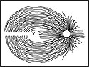
The temporal nerve fibers pass in an arcuate fashion superiorly and inferiorly around the fovea and travel in the optic nerve. These arcuate-shaped field defects arc around fixation and insert into the blind spot (the optic nerve is represented by the blind spot in the visual field). Unlike the temporal fibers, the nasal retinal fibers insert directly into the optic nerve nasally (Slide 1).
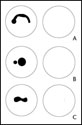
Glaucoma is the most common optic neuropathy producing nerve fiber layer defects, but any optic neuropathy (e.g., optic disc drusen, papilledema, anterior ischemic optic neuropathy) or retinal disease affecting retinal nerve fiber layer (e.g., branch retinal artery occlusion) may produce similar visual field loss patterns. An arcuate visual field defect may be superior or inferior, or a combination of both. Arcuate visual loss can become confluent altitudinal visual field loss. Generally, patients with arcuate visual field loss (Slide 2) have ophthalmoscopically visible pathologic changes in the retina or optic disc (e.g., glaucomatous cupping or sector optic atrophy, nerve fiber layer loss) that corresponds directly with the location, severity, and depth of the visual field loss.
Involvement of the papillomacular bundle (e.g., optic neuritis, Leber's hereditary optic neuropathy, macular disease) may produce a central scotoma (Slide 2) that may be unilateral or bilateral (depending on laterality of the process). A cecocentral scotoma is a central scotoma that extends to the blind spot (Slide 2). Bilateral central or cecocentral scotomas generally suggest a narrow differential diagnosis (e.g., toxic/nutritional or hereditary optic neuropathy), but other optic neuropathies (e.g., optic neuritis) or maculopathies may also cause similar field loss.
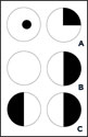
Previously, it was believed that inferonasal fibers crossing in the anterior optic chiasm loop traveled for a short course into the contralateral optic nerve (Wilbrand's knee). Clinically, a lesion at the junction of the optic nerve and chiasm was presumed to be the cause for an ipsilateral optic neuropathy (e.g., central scotoma) and a contralateral superotemporal visual field defect known as the junctional scotoma (Slide 3). The Wilbrand's knee, however, may be an artifact of enucleation rather than a distinct anatomic entity. Nevertheless, the clinical localizing value of the junctional scotoma (ipsilateral optic neuropathy with contralateral superotemporal field loss) remains valid. In addition to the traditional junctional scotoma, a strictly monocular but hemianopic (nasal or temporal unilateral hemianopic field loss) field defect also occurs at the junction (Slide 3). This monocular hemianopic visual field loss is referred to as junctional scotoma of Traquair to distinguish it from the superotemporal visual loss in the junctional scotoma. A bitemporal hemianopsia localizes to the optic chiasm (Slide 3). The bitemporal loss may be paracentral or peripheral, and complete or incomplete.
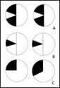
A homonymous hemianopsia localizes to the contralateral retrochiasmal pathway. The homonymous hemianopsia may be complete or incomplete (Slide 4). When incomplete, the homonymous field loss may be congruous (the same in each eye) or incongruous (different in each eye). Although a complete homonymous hemianopsia is lateralizing to the contralateral side, it is not further localizing by itself because the lesion can exist anywhere within the retrochiasmal pathway. The more congruous (or similar in appearance) the defect, the more posterior (e.g., occipital) in the retrochiasmal pathway is the lesion location. Conversely, the more incongruous (dissimilar) the homonymous hemianopsia, the more anterior (e.g., optic tract) the lesion is in the retrochiasmal pathway. The term congruity does not apply to a complete homonymous hemianopsia.
The retrochiasmal pathway is composed of the optic tract, the optic radiations, and the occipital cortex. Table 1 lists the localizing features for each of the retrochiasmal locations.
|
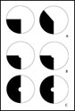
Several modalities are available for testing the visual field including confrontation testing, Amsler grid, tangent screen, manual kinetic testing (e.g., Goldmann technique) and automated static perimetry (e.g., Humphrey Field Analyzer [Zeiss], Octopus [Haag-Streit]). The advantages and disadvantages of each visual field strategy are listed in Table 2.
|
Several factors influence a clinician's decision to select one visual field test over another (i.e., Goldmann vs. Humphrey) including whether the central or peripheral visual field is being tested, whether qualitative shape vs. quantitative depth information is required, and whether patient-related factors exist that could limit reliability of testing (e.g., age, cooperation, and fatigue).
Central vs. Peripheral Testing
Small and paracentral visual field defects are tested best with confrontation, Amsler grid, or tangent screen techniques. Goldmann perimetry is performed with small and dim stimuli in the central area of interest to further define a central scotoma. Automated perimetry strategies are performed that concentrate on the central 10 degrees (e.g., Humphrey 10-2). If on the other hand the visual field defect is in the periphery (e.g., the monocular 60 degrees to 90 degrees temporal crescent from anterior calcarine cortex involvement), then Goldmann perimetry rather than an Amsler, tangent, or central automated field (10-2) should be performed.
Shape and Size of the Defect
The Goldmann perimeter provides qualitative information about the shape of a particular visual field defect (e.g., congruity, sloping vs. sharp margin). Automated perimetry of the central visual field (e.g., Humphrey 24-2) will detect homonymous or bitemporal hemianopic visual field loss. Generally, optic neuropathies (e.g., optic neuritis, ischemic optic neuropathy, papilledema, glaucoma) are evaluated and followed with automated perimetry of the central visual field. The widespread availability and speed of automated testing has supplanted manual perimetry in many institutions.
Patient-Related Factors
Active operator-based feedback is available in the Goldmann perimetry. This may be important for patients who are at the extremes of age (e.g., children or the elderly), patients who have issues of attention (e.g., fatigued, drowsy, or medicated patients) or concentration (e.g., hyperactive, inattentive, or distractible), or those who cannot reliably perform the test (e.g., mentally retarded, poor visual acuity, poor reliability indices).
Bibliography
- Donahue SP, Porter A. SITA visual field testing in children. J AAPOS. 2001; 5:114-117.
- Johnson CA, Keltner JL. Principles and techniques of the examination of the visual sensory system. In: Newman NJ, Miller NR, eds. Walsh and Hoyt's Clinical Neuro-Ophthalmology, 5th ed. Baltimore, MD: Williams and Wilkins; 1997:194.
- Keltner JL, Johnson CA, Spurr JO, Beck RW. Comparison of central and peripheral visual field properties in the optic neuritis treatment trial. Am J Ophthalmol. 1999;128:543-553.
- Khoury JM, Donahue SP, Lavin PJ, Tsai JC. Comparison of 24-2 and 30-2 perimetry in glaucomatous and nonglaucomatous optic neuropathies. J Neuroophthalmol. 1999;19:100-108.
- Sekhar GC, Naduvilath TJ, Lakkai M, et al. Sensitivity of Swedish interactive threshold algorithm compared with standard full threshold algorithm in Humphrey visual field testing. Ophthalmology. 2000;107:1303-1308.
- Stiebel-Kalish H, Lusky M, Yassur Y, et al. Swedish interactive thresholding algorithm fast for following visual fields in prepubertal idiopathic intracranial hypertension. Ophthalmology. 2004;111:1673-1675.
- Szatmary G, Biousse V, Newman NJ. Can Swedish interactive thresholding algorithm fast perimetry be used as an alternative to Goldmann perimetry in neuro-ophthalmic practice? Arch Ophthalmol. 2002;120:1162-1173.
- Trobe JD, Acosta PC, Krischer JP. A screening method for chiasmal visual-field defects. Arch Ophthalmol. 1981;99:264-271.
- Trope GE, Britton R. A comparison of Goldmann and Humphrey automated perimetry in patients with glaucoma. Br J Ophthalmol. 1987;71:489-493.
- Tschopp C, Safran AB, Laffi JL, et al. Automated static perimetry in the child: Methodologic and practical problems. Klin Monatsbl Augenheilkd. 1995;206:416-419.
- Tschopp C, Safran AB, Viviani P, et al. Automated visual field examination in children aged 5-8 years. Part I: Experimental validation of a testing procedure. Vision Res. 1998;38:2203-2010.